The Annotated JEPA

Elon Litman

January 27, 2026

JEPA: prediction in representation space

This post is a step-by-step, annotated, from-scratch walkthrough of Joint Embedding Predictive Architectures, or JEPAs. The goal is to do for JEPA what The Annotated Transformer did for the Transformer: build the full object, explain every moving part, and end with a working training loop. JEPA is Yann LeCun's proposed answer to a fundamental question in self-supervised learning: how do you train a model to understand the world without labels, without collapsing to trivial solutions, and without wasting capacity on irrelevant details?

The answer, elegant in principle and subtle in practice, is prediction in representation or latent space.

To keep the discussion concrete, the main running example is I‑JEPA, the image instantiationWhy images and video rather than text? LeCun argues that language is already a highly compressed, discrete representation of knowledge; predicting the next token requires modeling human communication patterns, not physical reality. Visual prediction, by contrast, demands understanding of persistence, occlusion, and dynamics. JEPA is designed for domains where pixel-level reconstruction wastes capacity on irrelevant details, a problem that does not arise in the same way for discrete tokens. We return to this near the end., introduced as a self-supervised method that learns semantic image representations by predicting representations of masked regions from visible contextSee Self-Supervised Learning from Images with a Joint-Embedding Predictive Architecture (2023). I-JEPA is a non-generative approach that avoids hand-crafted data augmentations entirely.. We will build I‑JEPA from scratch, then discuss its extension to video with V‑JEPA and V‑JEPA 2See V-JEPA: Latent Video Prediction for Visual Representation Learning (2024), and V-JEPA 2: Self-Supervised Video Models Enable Understanding, Prediction and Planning (2025)., and then examine LeJEPA, the latest attempt to replace engineering heuristics with a distributional regularizerSee LeJEPA: Provable and Scalable Self-Supervised Learning Without the Heuristics (2025)..

What follows is meant to be pedagogical. The implementation omits FlashAttention, gradient checkpointing, mixed-precision, and the batching strategies that make large-scale training feasible. These are engineering choices that would dominate a production codebase but are trivially separable from the mathematics.

The Problem

Self-supervised representation learning asks: how do you learn useful features without labels? You need an objective that captures meaningful structure and, without labels, finding one that actually works is the central difficulty of the field.

JEPA's answer: train by prediction, but predict in representation space. Why should this work at all, though?

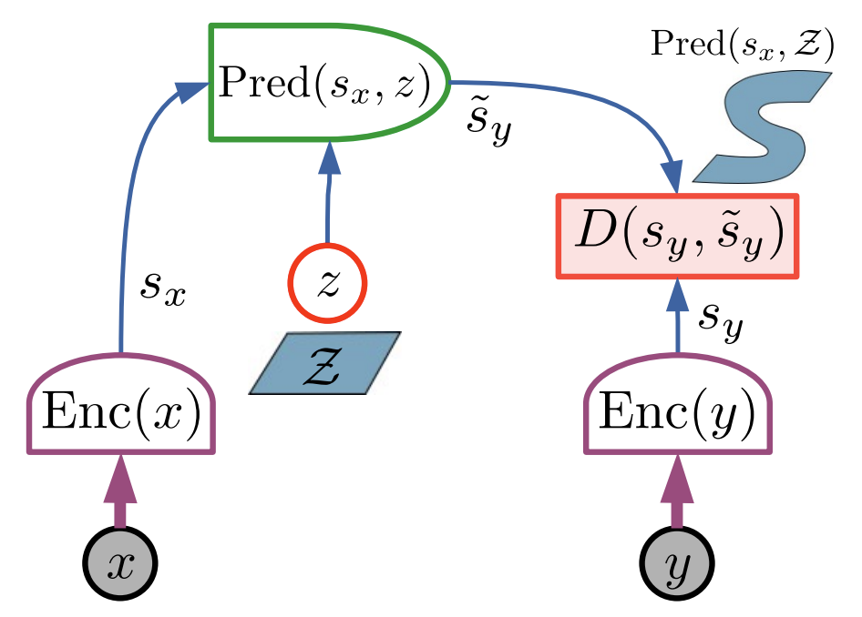
Suppose you see part of an image, the context $x$, and want to learn representations. Somewhere else in the image is a target region $y$ that you cannot see. An encoder maps $y$ to a representation $s_y$. A predictor takes your encoding of the context and outputs $\hat{s}_y$, its guess at what $s_y$ should be. Training minimizes the distance $D(\hat{s}_y, s_y)$.

Now ask: when can the predictor succeed? Only when the context encoding $s_x$ contains enough information to determine what $s_y$ must be. If you saw the hood of a car, predicting the representation of the wheels requires that your encoding of the hood captures this is a car. If you saw a face, predicting the representation of the hair requires that your encoding captures identity, pose, and lighting. The predictor cannot hallucinate structure that the context encoding lacks.

This is the forcing function. The context encoder must learn to extract features from $x$ that are predictive of $y$'s representation. These are exactly the semantic, structural features: object identity, spatial relationships, physical constraints. Pixel-level noise in $x$ does not help predict $s_y$, so the encoder learns to ignore it. What remains is what generalizes.

The target encoder has a complementary pressure. Its output $s_y$ must be predictable from context. If $s_y$ encoded random high-frequency texture, no amount of context would help predict it. So the target encoder learns to output representations that capture the shared structure between $x$ and $y$, the structure that makes prediction possible, rather than idiosyncratic details of $y$ alone.

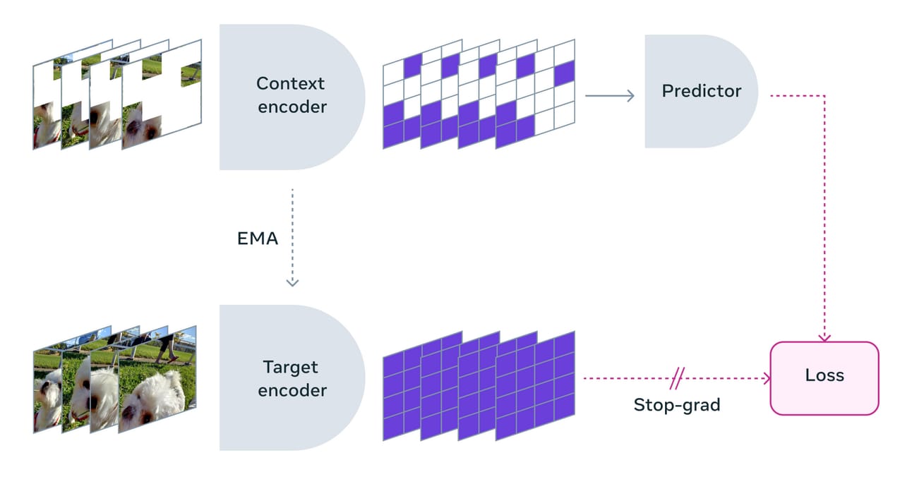
LeCun's position paper frames this as an energy-based formulationSee A Path Towards Autonomous Machine Intelligence (2022), OpenReview. LeCun frames JEPA as the foundation for world models that plan in latent space.: encode $x$ and $y$ into representations, predict one from the other, define energy as prediction error in that abstract space. The architecture factors into components we can implement and analyze: two encoders, one predictor, one distance function.

The JEPA Template

A JEPA starts from paired, semantically related views of the world. In the most general form, imagine triples $(x, y, z)$: $x$ is what you observe, $y$ is what you want to predict, and $z$ is an optional latent capturing unknown factors that make the prediction multimodal. The pairs $(x, y)$ are drawn from some joint distribution over observations. In image pretraining, $x$ might be visible patches and $y$ the masked patches of the same image; in video, $x$ is a clip prefix and $y$ is the continuation; in cross-modal settings, $x$ could be audio and $y$ the corresponding video. The only structural requirement is that knowing $x$ should constrain what $y$ can be.

LeCun's formulation adds an optional latent $z$ to handle multimodality in the predictive relationship. When multiple values of $y$ are consistent with the same $x$, the predictor conditions on $z$ to select among them. This matters for temporal prediction, where the future is genuinely uncertain, less so for masked image modeling, where the context typically determines the target up to noise.

The template has three parts. Encode both observations into a shared representation space:

$$ s_x = f_\theta(x), \quad s_y = f_{\bar\theta}(y) $$

The encoders $f_\theta$ and $f_{\bar\theta}$ can differ in architecture or parameter sharing. When $x$ and $y$ live in different modalities, they must differ; when they are the same modality, weight sharing is a design choice that trades inductive bias against flexibility.

Predict the target representation from the context representation:

$$\widehat{s}_y = g_\phi(s_x, z)$$

Minimize prediction error in representation space:

$$ \mathcal{L}(\theta, \bar\theta, \phi) = D(\widehat{s}_y, s_y) $$

The rest of this post instantiates these abstractions: defining $x$ and $y$ concretely for images, choosing architectures for the encoders and predictor, specifying the distance function $D$, and implementing the mechanism that prevents the trivial solution where all representations collapse to a constant.

Prediction vs. Reconstruction

Why predict in representation space rather than pixel space?

Consider two image patches that are semantically identical, same object, same meaning, but differ in hundreds of pixels due to lighting, texture, or JPEG artifacts. A reconstruction objective must explain all those differences. The model wastes capacity modeling high-entropy noise.

With JEPA, the target encoder can learn to output representations that discard nuisance details. When you regress to that representation, you push the model to capture what the encoder preserves, not what pixels happen to contain. I‑JEPA makes this explicit: the architecture resembles generative models, but the loss lives in embedding space, not input spaceAnalogous to perceptual losses (LPIPS) vs. pixel losses (MSE). Representation-space prediction lets the model focus on semantically meaningful features..

Collapse

The easiest way to minimize a matching loss? Output the same vector for everything. Then, loss goes to zero. But the representations become useless. This is the central failure mode of all joint embedding methods, and I‑JEPA addresses it directly: they use an asymmetric design between encoders.

The literature offers many anti-collapse strategiesSimCLR uses contrastive negatives. VICReg uses variance-invariance-covariance regularization. BYOL and SimSiam use stop-gradient. DINO/MoCo use EMA teachers. Each trades off differently.: contrastive negatives (expensive), explicit covariance constraints (tricky to tune), stop-gradient (surprisingly effective), or teacher-student encoders with exponential moving average updates (the I‑JEPA choice). I‑JEPA trains the context encoder and predictor by gradient descent, but updates the target encoder by exponential moving average (EMA) of the context encoder weights. Here is why this prevents collapse.

Consider what happens if both encoders are trained by gradient descent. The loss is $D(\hat{s}_y, s_y)$. If the target encoder can change freely, it will learn to output representations that are easy to predict, which means constant. The context encoder follows. Both converge to outputting the same vector for all inputs: loss zero, representations useless. EMA breaks this co-adaptation. The target encoder updates as

$$\theta_{\text{target}} \leftarrow m \theta_{\text{target}} + (1-m) \theta_{\text{context}}$$

with $m$ close to 1. This means the target encoder lags behind the context encoder. The target representations are stable on the timescale of a gradient step, so the context encoder cannot exploit fast-moving targets to find degenerate solutions. The context encoder must actually learn to predict what the (slowly evolving) target encoder outputs, which forces it to extract meaningful features.

Later we discuss LeJEPA, which tries to make collapse prevention principled rather than heuristic. For now, we focus on the classic I‑JEPA design.

Specializing JEPA to images

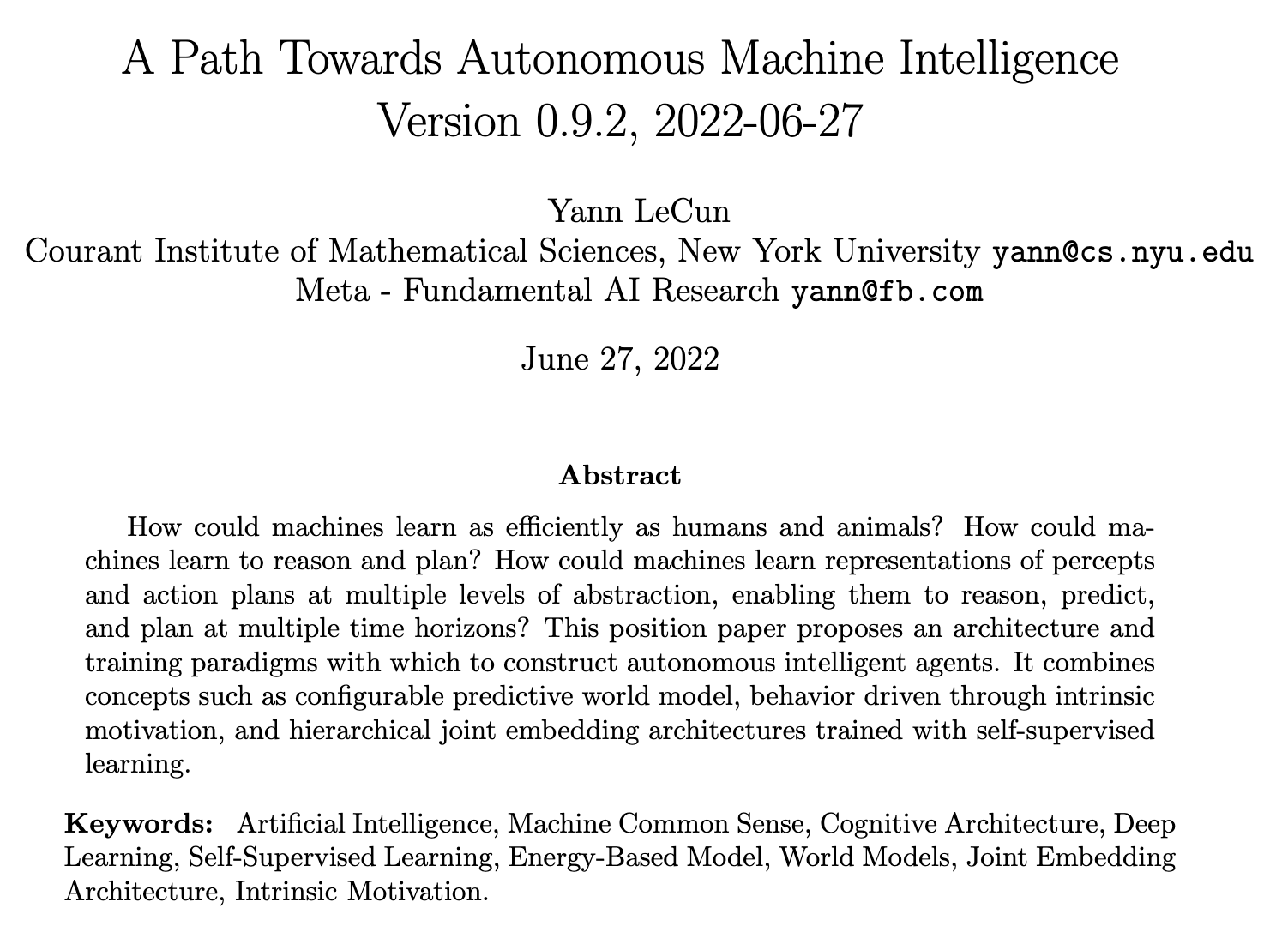
A JEPA needs paired views $x$ and $y$ that share semantics. For I‑JEPA, both come from the same image: $x$ is a large context block of patches, and $y$ consists of several smaller target blocks elsewhere in the image. The goal is to predict the representations of the target blocks from the context block. There are three key design choices in I‑JEPA that you should understand before writing any code.

The first choice is to represent the image as a sequence of patch tokens, following Vision TransformersSee Dosovitskiy et al., An Image is Worth 16x16 Words: Transformers for Image Recognition at Scale (2020). The ViT architecture splits images into fixed-size patches and processes them as a sequence.. A 224×224 image with 16×16 patches yields 196 tokens arranged in a 14×14 grid.

The second choice is the masking strategy. The paper states that to guide I‑JEPA toward semantic representations, it is crucial to predict target blocks that are sufficiently large in scale, and to use a context block that is sufficiently informative and spatially distributed. In the method section, the paper specifies typical mask sampling ranges: it commonly uses $M = 4$ target blocks, with an aspect ratio range $(0.75, 1.5)$ and a scale range $(0.15, 0.2)$. The context block is sampled with a scale range $(0.85, 1.0)$ and unit aspect ratio, and any overlap between targets and context is removed to keep the prediction task non-trivial.

The third choice is where masking happens for targets. Target blocks are obtained by masking the output of the target encoder, not the input. The target encoder sees the full image and produces high-level representations; we then select which representations to predict. The paper says this distinction is crucial to ensure the target representations are of a high semantic levelThis is computationally heavier than masking inputs for both views, but necessary for correctness. Since ViT uses global attention, a patch's representation depends on the full image context. Running the target encoder only on target patches would change what those representations mean..

These are not arbitrary implementation details. They are the entire point of I‑JEPA's inductive bias, replacing hand-designed multi-view augmentations with a structured prediction task.

The full Image‑JEPA architecture

We will implement three networks.

The context encoder (also called the student) is a Vision Transformer that processes only the visible context patches and produces a set of context embeddings.

The target encoder (also called the teacher) is another Vision Transformer that processes the full image and produces embeddings for all patches. Its weights are not updated by gradients; they are updated by exponential moving average of the context encoder weights.

The predictor is a smaller Transformer that takes the context embeddings and a set of mask tokens corresponding to the target patch positions, and produces predicted embeddings for those target positions. The method description says the predictor takes as input the context encoder output plus a mask token for each patch to predict, with the mask token parameterized by a shared learnable vector and an added positional embedding.

The loss is mean squared error between predicted patch representations and the target encoder's patch representations for the target blocks. This is the distance function $D$ from the JEPA template:

$$D(\hat{s}_y, s_y) = \|\hat{s}_y - s_y\|^2_2$$

A PyTorch implementation

The implementation is broken into pieces; you should be able to read it from top to bottom. Throughout, we will use these conventions: images have shape $(B, C, H, W)$ and patch tokens have shape $(B, N, D)$, where $N$ is the number of patches and $D$ is the embedding dimension. Whenever we select a subset of patches, we will represent that subset as a vector of indices into the $N$ patches and we will implement absolute positional embeddings for simplicity.

Imports and small helpers

import math
import random
from dataclasses import dataclass
from typing import List, Optional, Tuple

import torch
import torch.nn as nn
import torch.nn.functional as F

Patch embedding

A standard Vision Transformer creates patch tokens with a strided convolution. Each patch becomes a vector in $\mathbb{R}^D$.

class PatchEmbed(nn.Module):
    """
    Converts an image to a sequence of patch embeddings.

    Input:  (B, C, H, W)
    Output: (B, N, D) where N = (H / P) * (W / P)
    """
    def __init__(
        self,
        img_size: int = 224,
        patch_size: int = 16,
        in_chans: int = 3,
        embed_dim: int = 768,
    ):
        super().__init__()
        assert img_size % patch_size == 0, "img_size must be divisible by patch_size"

        self.img_size = img_size
        self.patch_size = patch_size
        self.grid_size = img_size // patch_size
        self.num_patches = self.grid_size * self.grid_size

        self.proj = nn.Conv2d(
            in_channels=in_chans,
            out_channels=embed_dim,
            kernel_size=patch_size,
            stride=patch_size,
            bias=True,
        )

    def forward(self, x: torch.Tensor) -> torch.Tensor:
        x = self.proj(x)                 # (B, D, G, G)
        x = x.flatten(2).transpose(1, 2) # (B, N, D)
        return x

The only non-obvious line is the reshape. After the convolution you have $(B, D, G, G)$. Flattening dimensions 2 and 3 yields $(B, D, N)$. Transposing gives the usual token format $(B, N, D)$.

The Transformer block

I‑JEPA uses Vision Transformers for the encoders and for the predictor. We will implement a standard pre-norm Transformer block, which is close to what most practical ViTs usePre-norm (LayerNorm before attention/MLP) is more stable for training deep transformers than post-norm (LayerNorm after). See Xiong et al., On Layer Normalization in the Transformer Architecture (2020)..

First, multi-head self-attention:

class MultiHeadSelfAttention(nn.Module):
    def __init__(
        self,
        dim: int,
        num_heads: int,
        attn_drop: float = 0.0,
        proj_drop: float = 0.0,
    ):
        super().__init__()
        assert dim % num_heads == 0, "dim must be divisible by num_heads"

        self.dim = dim
        self.num_heads = num_heads
        self.head_dim = dim // num_heads
        self.scale = self.head_dim ** -0.5

        self.qkv = nn.Linear(dim, 3 * dim, bias=True)
        self.attn_drop = nn.Dropout(attn_drop)
        self.proj = nn.Linear(dim, dim, bias=True)
        self.proj_drop = nn.Dropout(proj_drop)

    def forward(self, x: torch.Tensor) -> torch.Tensor:
        """
        x: (B, T, D)
        """
        B, T, D = x.shape

        qkv = self.qkv(x)                              # (B, T, 3D)
        qkv = qkv.reshape(B, T, 3, self.num_heads, self.head_dim)
        qkv = qkv.permute(2, 0, 3, 1, 4)               # (3, B, H, T, Hd)

        q, k, v = qkv[0], qkv[1], qkv[2]               # (B, H, T, Hd) each

        attn = (q @ k.transpose(-2, -1)) * self.scale  # (B, H, T, T)
        attn = attn.softmax(dim=-1)
        attn = self.attn_drop(attn)

        out = attn @ v                                 # (B, H, T, Hd)
        out = out.transpose(1, 2).reshape(B, T, D)      # (B, T, D)

        out = self.proj(out)
        out = self.proj_drop(out)
        return out

Then the MLP:

class MLP(nn.Module):
    def __init__(self, dim: int, hidden_dim: int, drop: float = 0.0):
        super().__init__()
        self.fc1 = nn.Linear(dim, hidden_dim)
        self.act = nn.GELU()
        self.fc2 = nn.Linear(hidden_dim, dim)
        self.drop = nn.Dropout(drop)

    def forward(self, x: torch.Tensor) -> torch.Tensor:
        x = self.fc1(x)
        x = self.act(x)
        x = self.drop(x)
        x = self.fc2(x)
        x = self.drop(x)
        return x

Then the Transformer block:

class TransformerBlock(nn.Module):
    def __init__(
        self,
        dim: int,
        num_heads: int,
        mlp_ratio: float = 4.0,
        attn_drop: float = 0.0,
        drop: float = 0.0,
    ):
        super().__init__()
        self.norm1 = nn.LayerNorm(dim)
        self.attn = MultiHeadSelfAttention(
            dim=dim,
            num_heads=num_heads,
            attn_drop=attn_drop,
            proj_drop=drop,
        )
        self.norm2 = nn.LayerNorm(dim)
        self.mlp = MLP(dim=dim, hidden_dim=int(dim * mlp_ratio), drop=drop)

    def forward(self, x: torch.Tensor) -> torch.Tensor:
        x = x + self.attn(self.norm1(x))
        x = x + self.mlp(self.norm2(x))
        return x

You can now build a ViT encoder by stacking these blocks.

A ViT encoder that can process a subset of patches

I‑JEPA's efficiency comes from letting the context encoder process only visible context patches. To model that, we write an encoder that can optionally select patches by index before running the Transformer:

class ViTEncoder(nn.Module):
    """
    Minimal ViT-style patch encoder.

    This version does not use a CLS token. The I-JEPA method section describes
    patch-level representations and does not require CLS during pretraining.
    """
    def __init__(
        self,
        img_size: int = 224,
        patch_size: int = 16,
        in_chans: int = 3,
        embed_dim: int = 768,
        depth: int = 12,
        num_heads: int = 12,
        mlp_ratio: float = 4.0,
        drop: float = 0.0,
        attn_drop: float = 0.0,
    ):
        super().__init__()
        self.patch_embed = PatchEmbed(img_size, patch_size, in_chans, embed_dim)
        self.num_patches = self.patch_embed.num_patches

        self.pos_embed = nn.Parameter(torch.zeros(1, self.num_patches, embed_dim))
        nn.init.trunc_normal_(self.pos_embed, std=0.02)

        self.blocks = nn.ModuleList([
            TransformerBlock(
                dim=embed_dim,
                num_heads=num_heads,
                mlp_ratio=mlp_ratio,
                attn_drop=attn_drop,
                drop=drop,
            )
            for _ in range(depth)
        ])
        self.norm = nn.LayerNorm(embed_dim)

    def forward(self, images: torch.Tensor, patch_indices: Optional[torch.Tensor] = None) -> torch.Tensor:
        """
        images: (B, C, H, W)
        patch_indices: None or a 1D tensor of indices into the patch sequence

        Returns: (B, T, D)
        """
        x = self.patch_embed(images)  # (B, N, D)

        if patch_indices is None:
            x = x + self.pos_embed
        else:
            if patch_indices.dim() != 1:
                raise ValueError("patch_indices must be a 1D tensor in this minimal implementation")
            x = x[:, patch_indices, :] + self.pos_embed[:, patch_indices, :]

        for blk in self.blocks:
            x = blk(x)

        x = self.norm(x)
        return x

There is a deliberate limitation: patch_indices is shared across the batch. In real training, each image has different masks, so you either vectorize with padding and attention masks or you loop over samples. For pedagogy, we will loop.

Block mask sampling

Now we implement the core I‑JEPA view construction: sample multiple target blocks and one context block, then remove overlap. The paper describes this procedure and provides typical ranges: four target blocks with scale in the range $(0.15, 0.2)$ and aspect ratio $(0.75, 1.5)$, one context block with scale $(0.85, 1.0)$ and unit aspect ratio, and then remove overlap between target and context.

We will implement a mask generator that returns patch indices:

def _sample_block_on_grid(
    grid_size: int,
    scale_range: Tuple[float, float],
    aspect_ratio_range: Tuple[float, float],
) -> Tuple[int, int, int, int]:
    """
    Samples a rectangle on a grid_size x grid_size patch grid.

    Returns (top, left, height, width) in patch coordinates.
    """
    G = grid_size
    N = G * G

    scale = random.uniform(scale_range[0], scale_range[1])
    aspect = random.uniform(aspect_ratio_range[0], aspect_ratio_range[1])

    area = scale * N
    w = int(round(math.sqrt(area * aspect)))
    h = int(round(math.sqrt(area / aspect)))

    w = max(1, min(G, w))
    h = max(1, min(G, h))

    top = random.randint(0, G - h)
    left = random.randint(0, G - w)
    return top, left, h, w


def _rect_to_indices(grid_size: int, top: int, left: int, h: int, w: int) -> torch.Tensor:
    """
    Converts a rectangle to flat patch indices in row major order.
    """
    rows = torch.arange(top, top + h)
    cols = torch.arange(left, left + w)
    rr, cc = torch.meshgrid(rows, cols, indexing="ij")
    idx = rr * grid_size + cc
    return idx.flatten()

Now the generator:

@dataclass
class IJEPAMasks:
    context_idx: torch.Tensor
    target_blocks: List[torch.Tensor]


class IJEPAMaskGenerator:
    def __init__(
        self,
        grid_size: int,
        num_targets: int = 4,
        target_scale: Tuple[float, float] = (0.15, 0.20),
        target_aspect: Tuple[float, float] = (0.75, 1.50),
        context_scale: Tuple[float, float] = (0.85, 1.00),
        context_aspect: Tuple[float, float] = (1.00, 1.00),
    ):
        self.grid_size = grid_size
        self.num_targets = num_targets
        self.target_scale = target_scale
        self.target_aspect = target_aspect
        self.context_scale = context_scale
        self.context_aspect = context_aspect

    def __call__(self) -> IJEPAMasks:
        G = self.grid_size

        target_blocks: List[torch.Tensor] = []
        target_union = torch.zeros(G * G, dtype=torch.bool)

        for _ in range(self.num_targets):
            top, left, h, w = _sample_block_on_grid(G, self.target_scale, self.target_aspect)
            idx = _rect_to_indices(G, top, left, h, w)
            target_blocks.append(idx)
            target_union[idx] = True

        c_top, c_left, c_h, c_w = _sample_block_on_grid(G, self.context_scale, self.context_aspect)
        context_idx = _rect_to_indices(G, c_top, c_left, c_h, c_w)

        keep = ~target_union[context_idx]
        context_idx = context_idx[keep]

        return IJEPAMasks(context_idx=context_idx, target_blocks=target_blocks)

This generator embodies the paper's method section description of how the targets and context are sampled and how overlap is removed. From a JEPA viewpoint, this is the definition of $x$ and the definition of which parts of $y$ we are trying to predict.

The predictor and mask tokens

In I‑JEPA, the predictor receives context embeddings plus mask tokens that mark the target positions we want it to predict. The paper describes the mask tokens as a shared learnable vector with positional embedding added.

A minimal design is to implement the predictor as a small Transformer that processes a concatenated sequence: the input sequence is the context tokens followed by mask tokens, one per target patch position, each augmented with the positional embedding for that patch position. The output sequence is the same length, and we read out the final tokens corresponding to the target positions.

class IJEPA_Predictor(nn.Module):
    def __init__(
        self,
        embed_dim: int,
        depth: int = 6,
        num_heads: int = 12,
        mlp_ratio: float = 4.0,
        drop: float = 0.0,
        attn_drop: float = 0.0,
    ):
        super().__init__()
        self.mask_token = nn.Parameter(torch.zeros(1, 1, embed_dim))
        nn.init.trunc_normal_(self.mask_token, std=0.02)

        self.blocks = nn.ModuleList([
            TransformerBlock(
                dim=embed_dim,
                num_heads=num_heads,
                mlp_ratio=mlp_ratio,
                attn_drop=attn_drop,
                drop=drop,
            )
            for _ in range(depth)
        ])
        self.norm = nn.LayerNorm(embed_dim)

    def forward(self, context_tokens: torch.Tensor, target_pos_embed: torch.Tensor) -> torch.Tensor:
        """
        context_tokens: (B, Nc, D)
        target_pos_embed: (B, Nt, D)

        Returns: (B, Nt, D)
        """
        B, Nc, D = context_tokens.shape
        _, Nt, _ = target_pos_embed.shape

        mask_tokens = self.mask_token.expand(B, Nt, D) + target_pos_embed
        x = torch.cat([context_tokens, mask_tokens], dim=1)

        for blk in self.blocks:
            x = blk(x)

        x = self.norm(x)
        pred_target = x[:, Nc:, :]
        return pred_target

There are two conceptual reasons this works. First, self-attention lets each mask token attend to all context tokens, so information flows from what the model saw to what it must predict. Second, adding positional embeddings to the mask tokens tells the predictor where in the image the unknown region lives; without this, all target positions would be indistinguishable.

Wiring the full model

Now we implement the JEPA template exactly. The target encoder produces $s_y$ for all patches. The mask generator chooses a context subset and several target subsets. The context encoder encodes only the context subset into $s_x$. For each target block, the predictor outputs $\widehat{s}_y$ at those positions. The loss is mean squared error between predicted embeddings and target embeddings on the target positions.

The target encoder is updated by exponential moving average, rather than gradients:

$$\theta_{\text{target}} \leftarrow m \theta_{\text{target}} + (1-m) \theta_{\text{context}}$$

I‑JEPA states this explicitly and notes that they find an EMA target encoder essential in their settingHere $m$ is typically $0.996$ to $1.0$. This creates a slowly-evolving teacher that provides stable targets..

class IJEPAModel(nn.Module):
    def __init__(
        self,
        img_size: int = 224,
        patch_size: int = 16,
        in_chans: int = 3,
        embed_dim: int = 768,
        enc_depth: int = 12,
        enc_heads: int = 12,
        pred_depth: int = 6,
        pred_heads: int = 12,
        mlp_ratio: float = 4.0,
    ):
        super().__init__()

        self.context_encoder = ViTEncoder(
            img_size=img_size,
            patch_size=patch_size,
            in_chans=in_chans,
            embed_dim=embed_dim,
            depth=enc_depth,
            num_heads=enc_heads,
            mlp_ratio=mlp_ratio,
        )

        self.target_encoder = ViTEncoder(
            img_size=img_size,
            patch_size=patch_size,
            in_chans=in_chans,
            embed_dim=embed_dim,
            depth=enc_depth,
            num_heads=enc_heads,
            mlp_ratio=mlp_ratio,
        )

        self._init_teacher_from_student()

        self.predictor = IJEPA_Predictor(
            embed_dim=embed_dim,
            depth=pred_depth,
            num_heads=pred_heads,
            mlp_ratio=mlp_ratio,
        )

        G = self.context_encoder.patch_embed.grid_size
        self.mask_generator = IJEPAMaskGenerator(grid_size=G)

    @torch.no_grad()
    def _init_teacher_from_student(self) -> None:
        for p_t, p_s in zip(self.target_encoder.parameters(), self.context_encoder.parameters()):
            p_t.data.copy_(p_s.data)
        for p in self.target_encoder.parameters():
            p.requires_grad_(False)

    @torch.no_grad()
    def ema_update_teacher(self, momentum: float) -> None:
        """
        Teacher update: theta_bar <- m * theta_bar + (1 - m) * theta
        """
        for p_t, p_s in zip(self.target_encoder.parameters(), self.context_encoder.parameters()):
            p_t.data.mul_(momentum).add_(p_s.data, alpha=(1.0 - momentum))

    def forward(self, images: torch.Tensor) -> torch.Tensor:
        """
        Computes the I-JEPA loss on a batch.

        This version loops over samples for clarity, since masks differ per image.
        """
        B = images.shape[0]
        device = images.device

        with torch.no_grad():
            target_tokens_all = self.target_encoder(images, patch_indices=None)  # (B, N, D)

        pos_embed = self.context_encoder.pos_embed  # (1, N, D)

        total_loss = 0.0
        total_blocks = 0

        for b in range(B):
            masks = self.mask_generator()
            context_idx = masks.context_idx.to(device)

            context_tokens = self.context_encoder(images[b:b+1], patch_indices=context_idx)  # (1, Nc, D)

            for block_idx in masks.target_blocks:
                block_idx = block_idx.to(device)

                target_block = target_tokens_all[b:b+1, block_idx, :]  # (1, Nt, D)
                target_pos = pos_embed[:, block_idx, :]                # (1, Nt, D)

                pred_block = self.predictor(context_tokens, target_pos) # (1, Nt, D)

                loss = F.mse_loss(pred_block, target_block, reduction="mean")
                total_loss += loss
                total_blocks += 1

        return total_loss / max(1, total_blocks)

This is the clearest embodiment of I‑JEPA's method description: the predictor is applied once per target block, conditioned on the target locations, and the loss averages over those predicted patch representationsA subtlety: since target blocks have variable sizes, averaging MSE per block weights patches in smaller blocks more heavily than patches in larger blocks. To define energy strictly as average error per patch, you would sum squared errors and divide by total patch count. In practice, stochastic sampling averages this out..

The architecture is complete. What remains is training.

Training loop and the EMA momentum schedule

I‑JEPA uses an EMA teacher update. In practice, you choose a momentum $m$ close to 1, and often increase it toward 1 across training. Different papers use linear or cosine schedules. The essential requirement is that the teacher should evolve more slowly than the student. Here is a schedule helper and a minimal training loop:

def cosine_schedule(start: float, end: float, step: int, total_steps: int) -> float:
    if total_steps <= 1:
        return end
    t = step / (total_steps - 1)
    return end - (end - start) * (0.5 * (1 + math.cos(math.pi * t)))


def momentum_schedule(step: int, total_steps: int, start_m: float = 0.996, end_m: float = 1.0) -> float:
    return cosine_schedule(start_m, end_m, step, total_steps)


def train_ijepa(
    model: IJEPAModel,
    dataloader,
    epochs: int,
    lr: float = 1e-4,
    weight_decay: float = 0.05,
    device: str = "cuda",
) -> None:
    model.to(device)
    model.train()

    params = list(model.context_encoder.parameters()) + list(model.predictor.parameters())
    opt = torch.optim.AdamW(params, lr=lr, weight_decay=weight_decay)

    total_steps = epochs * len(dataloader)
    global_step = 0

    for epoch in range(epochs):
        for batch in dataloader:
            images = batch[0].to(device)

            loss = model(images)

            opt.zero_grad(set_to_none=True)
            loss.backward()
            opt.step()

            m = momentum_schedule(global_step, total_steps)
            model.ema_update_teacher(momentum=m)

            if global_step % 50 == 0:
                print(f"step={global_step} epoch={epoch} loss={loss.item():.6f} momentum={m:.6f}")

            global_step += 1

Production code adds mixed precision, gradient clipping, distributed training, and careful batching (uniform mask sizes within each batch, for instance, so you can vectorize the forward pass rather than loop over samples). These are engineering choices orthogonal to the method.

The EMA update and momentum schedule are not orthogonal. As explained earlier, EMA is what prevents collapse by making the target encoder lag behind the context encoder. The schedule (increasing $m$ toward 1) makes the teacher increasingly stable as training progresses. These are design choices that change whether the method works, not merely how fast it trains.

How to use a pretrained I‑JEPA encoder

After pretraining, you usually want a single embedding per image. A common approach is to use the target encoder and average-pool its patch embeddings. This gives a global representation that you can feed into a linear classifier, a nearest-neighbor evaluation, or a downstream fine-tuning pipeline.

@torch.no_grad()
def encode_global_target(model: IJEPAModel, images: torch.Tensor) -> torch.Tensor:
    model.eval()
    tokens = model.target_encoder(images, patch_indices=None)  # (B, N, D)
    return tokens.mean(dim=1)                                  # (B, D)

This is not the only choice. You might use a CLS token during fine-tuning, you might use attention pooling, or you might keep patch embeddings for dense prediction tasks. JEPA pretraining has already organized patch representations in a way that makes downstream adaptation easier.

Sanity checks

A JEPA implementation can silently fail. Unlike supervised learning, where accuracy directly measures what you care about, or language modeling, where perplexity on held-out text correlates reasonably well with downstream capabilities, JEPA's training loss is not commensurate with representation quality. The loss measures prediction error in representation space, but what matters is whether those representations are useful for downstream tasks. In JEPA, the relationship between the self-supervised objective and downstream utility is mediated by the representation space itself, and that mediation is not guaranteed to be monotonic or even predictable from loss alone.

Thus, you cannot debug a JEPA by watching loss decrease. You need auxiliary diagnostics. Here are three checks you can implement as short diagnostic functions. First, verify that the teacher is not receiving gradients:

def assert_teacher_frozen(model: IJEPAModel) -> None:
    for p in model.target_encoder.parameters():
        assert p.requires_grad is False

Second, monitor representation variance across a batch. Collapse often shows up as near-zero varianceA healthy representation space should have variance roughly proportional to the embedding dimension. If variance drops below $0.1$ or so, collapse is likely occurring. You can also use VICReg to explicitly regularize this quantity.:

@torch.no_grad()
def embedding_variance(tokens: torch.Tensor) -> float:
    return tokens.std(dim=0).mean().item()

Third, verify that context and target regions truly do not overlap in patch indices. If overlap exists, the task becomes too easy and may distort the learned representation. The paper explicitly removes overlap for a non-trivial task. This kind of instrumentation rarely appears in papers but often allows you to diagnose a failing run quickly.

What makes I‑JEPA a JEPA

Now that we have code, it is worth re-stating the conceptual structure. The joint embedding part is that both the student and the teacher produce embeddings of the same object, the image, and the learning signal is a comparison in embedding space. The predictive part is that the student is not matching a second view of the entire image. It is predicting embeddings of masked target regions from embeddings of visible context regions, using an explicit predictor network conditioned on positional information. The non-generative part is that there is no pixel decoder. The model is not asked to reconstruct tokens or pixels. The loss is on embeddings.

V‑JEPA: extending JEPA to video

Video amplifies the case for representation-space prediction: frames are redundant, pixels are noisy, and the dynamics that matter live in abstraction.

Before V‑JEPA, there was MC‑JEPA (Motion-Content JEPA), published in July 2023See MC-JEPA: A Joint-Embedding Predictive Architecture for Self-Supervised Learning of Motion and Content Features (2023). MC-JEPA uses a shared encoder to simultaneously learn motion dynamics and static content features from video.. MC‑JEPA introduced a key insight: video contains two intertwined signals, motion (how things change) and content (what things are), and a JEPA can learn to disentangle them using a shared encoder. This was an important stepping stone, demonstrating that JEPA-style prediction could handle the additional complexity of temporal data.

V‑JEPA builds on this foundation by extending the same principle (predict representations, not pixels) to the full spatiotemporal domainSee V-JEPA: Latent Video Prediction for Visual Representation Learning (2024). The paper demonstrates that predicting in latent space significantly outperforms pixel-space prediction objectives for video..

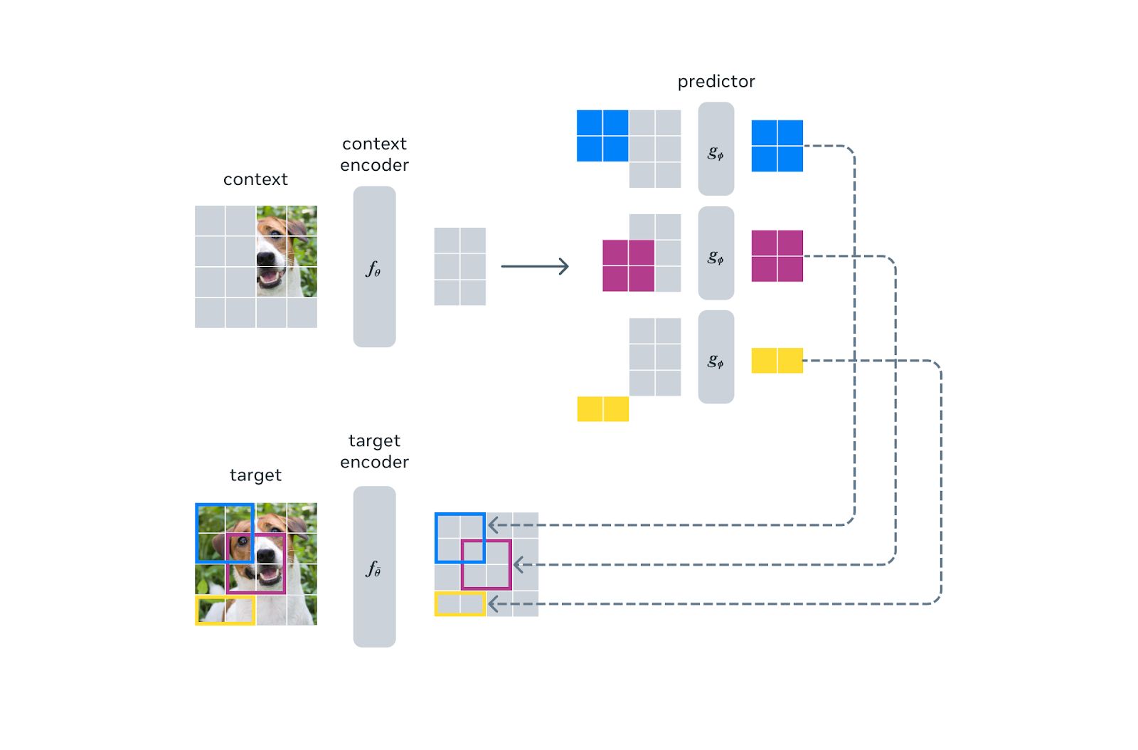
The key insight is that video is even more wasteful to reconstruct than images. Consecutive frames are highly redundant; much of the pixel-level detail is irrelevant noise; and modeling temporal dynamics at the pixel level requires enormous capacity. V‑JEPA sidesteps all of this by masking spatiotemporal regions of a video and predicting their representations from the visible context.

Architecturally, V‑JEPA uses a Vision Transformer backbone that processes video as a sequence of spatiotemporal patches. A video is divided into a 3D grid of patches (spatial × spatial × temporal), each patch is embedded, and the encoder operates over this sequence. The masking strategy is adapted accordingly: instead of masking 2D blocks as in I‑JEPA, V‑JEPA masks 3D spatiotemporal blocksEarlier video methods like VideoMAE used tube masking, where the same spatial region is masked across all frames. V‑JEPA moved away from this: random 3D blocks with limited temporal extent force the model to learn actual dynamics rather than relying on the tube assumption., forcing the model to reason about temporal coherence and motion.

The same EMA teacher framework applies: the context encoder and predictor are trained by gradient descent, while the target encoder provides stable regression targets via exponential moving average updates. The loss remains prediction error in representation space.

V‑JEPA's results demonstrate that this approach learns strong video representations without requiring temporal augmentations, optical flow computation, or any form of pixel-level reconstruction. The representations transfer well to downstream video understanding tasks like action recognition.

V‑JEPA 2: from representation learning to planning

V‑JEPA 2 takes the JEPA framework further by showing that the same architecture can support not just representation learning, but also prediction and planningSee V-JEPA 2: Self-Supervised Video Models Enable Understanding, Prediction and Planning (2025). This work demonstrates that a single pretrained model can serve multiple purposes: frozen features for classification, fine-tuned predictions for forecasting, and latent planning for embodied agents..

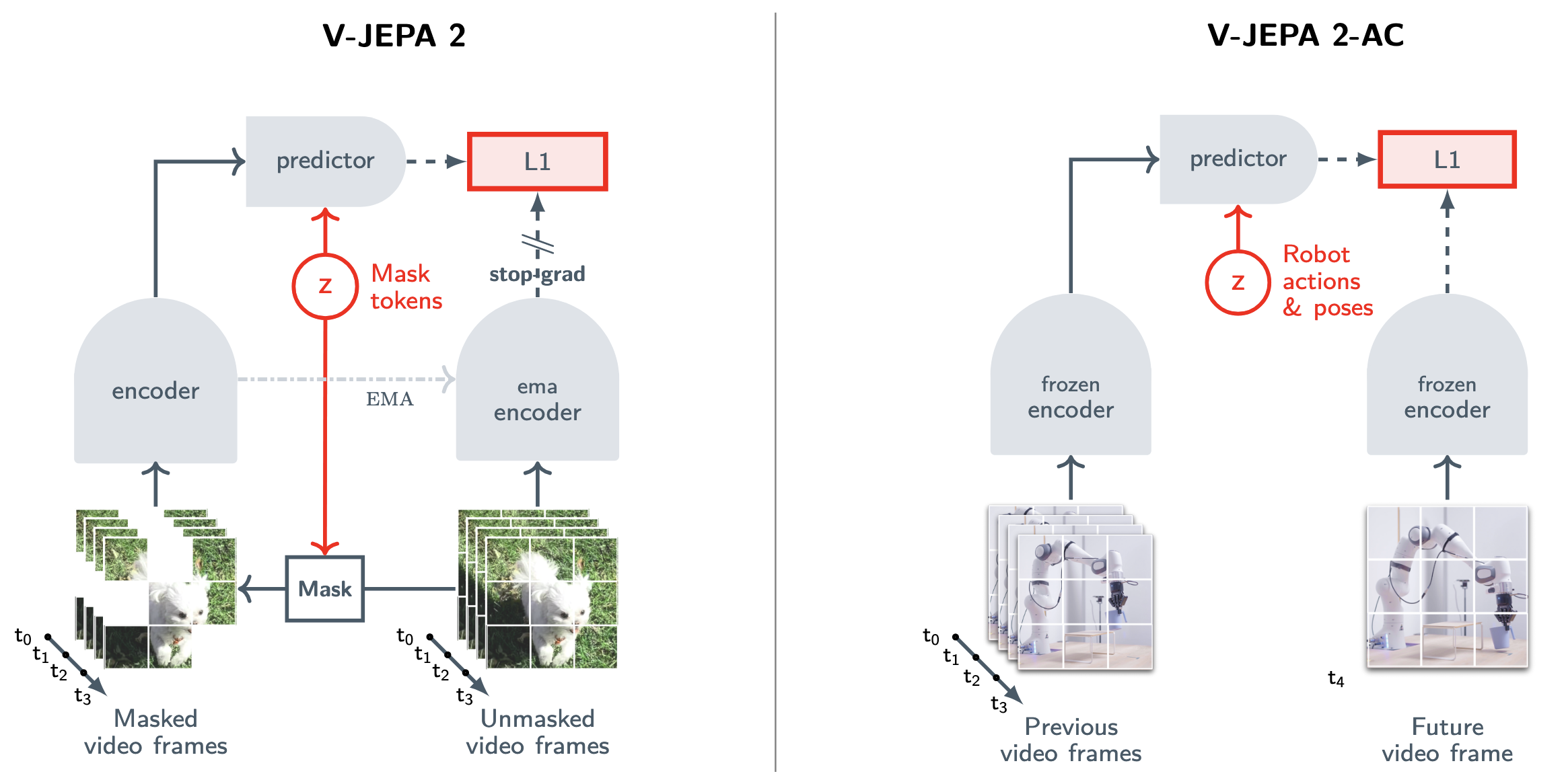
V-JEPA 2 architecture and V-JEPA 2-AC for action-conditioned planning

The conceptual leap is significant. V‑JEPA 2 is trained on a massive corpus of video data using the same JEPA objective (left side of the figure), but the resulting model can then be used in three distinct modes.

In understanding mode, the pretrained encoder produces features that transfer to video classification and action recognition tasks, much like the original V‑JEPA. The model has learned to organize video into meaningful representations.

In prediction mode, the model generates future latent states conditioned on past observations. Given a video prefix, the predictor outputs what comes next in representation space. Thus, it is not hallucinating pixels. Rather, it is forecasting the abstract state of the world.

Planning mode is where representation-space prediction pays its largest dividend, and this requires action-conditioning. The right side of the figure shows V‑JEPA 2-AC: the pretrained encoder is frozen, and the predictor is fine-tuned to take robot actions and poses as input (the latent $z$ in the JEPA template). Given the current visual state and a candidate action, the predictor outputs the representation of what the world will look like after that action. This is a learned dynamics model in latent space.

An agent equipped with this model can plan by search. To reach a goal state, it considers candidate action sequences, rolls out each one by repeatedly applying the predictor, and evaluates which trajectory gets closest to the goal representation. The search is tractable precisely because the representation has compressed away irrelevant details: no need to hallucinate textures, lighting, or camera noise for hypothetical futures. V‑JEPA 2 demonstrates that the same core idea, predict representations rather than reconstructions, extends from masked image patches to real-time understanding, multi-step forecasting, and goal-directed planning. What began as a self-supervised pretraining objective may plausibly become a foundation for systems that can imagine before they act!

LeJEPA: a JEPA without heuristics

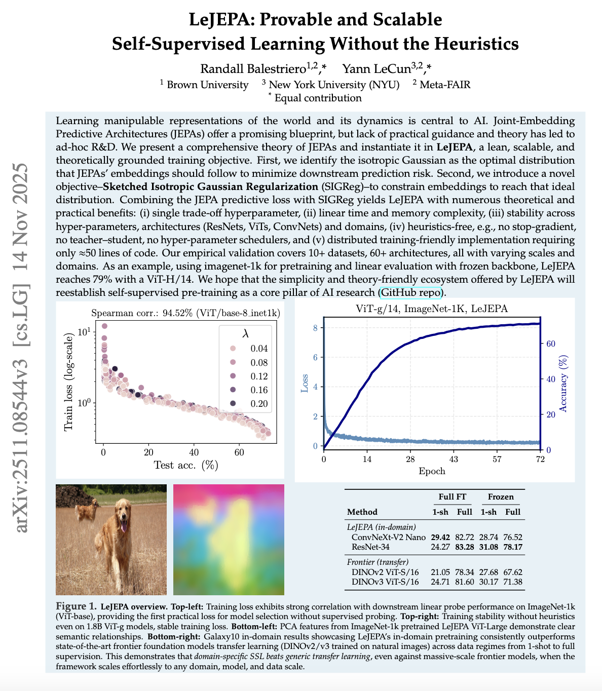
LeJEPA: Provable and Scalable Self-Supervised Learning Without the Heuristics

LeJEPA deserves a careful explanation because it is motivated by a critique of exactly the kind of design we just implemented. LeJEPA is presented as a lean, scalable, theoretically grounded training objective that aims to make JEPA training stable without many common heuristics. The abstract explicitly advertises "no stop-gradient, no teacher-student, no hyperparameter schedulers," and it claims linear time and memory complexity and a single tradeoff hyperparameter.

The core idea in LeJEPA is to treat "avoiding collapse" as a distribution matching problem.

The paper argues that, to minimize downstream prediction risk, JEPA embeddings should follow an isotropic Gaussian distribution, and it introduces Sketched Isotropic Gaussian Regularization, abbreviated SIGReg, as a way to push the embedding distribution toward that targetSIGReg uses random projections and statistical tests to enforce distributional properties without computing full covariance matrices. This makes it scale linearly with batch size and embedding dimension..

To understand what that means, start from the following perspective: a collapsed representation is degenerate because it has low spread. If all embeddings are nearly identical, their distribution is extremely concentrated. An isotropic Gaussian, by contrast, is maximally spread in a symmetric way: variance is equal in every direction and dimensions are uncorrelated in the idealized sense. LeJEPA claims that enforcing an isotropic Gaussian distribution is both theoretically optimal for downstream risk and practically effective at preventing collapse. Now, the question is how to enforce that distribution in high dimensions.

LeJEPA's SIGReg mechanism works as follows. Take a batch of embeddings $\{s_i\}$ in $\mathbb{R}^D$. Sample a random direction $w \in \mathbb{R}^D$. Project each embedding onto that direction to get scalars $\{w^\top s_i\}$. If the embeddings were truly isotropic Gaussian, these projected scalars would be univariate Gaussian. So compute a statistical test (the paper uses characteristic function matching) that measures how far the empirical distribution of $\{w^\top s_i\}$ deviates from Gaussian. Average over many random directions $w$. This gives a loss that penalizes non-Gaussianity.

The mathematical justification is the Cramér-Wold theorem: a distribution in $\mathbb{R}^D$ is uniquely determined by its one-dimensional projectionsThe Cramér-Wold theorem states that a probability distribution in $\mathbb{R}^d$ is uniquely determined by its one-dimensional projections. This is the theoretical foundation for sliced Wasserstein distances and related methods.. If every 1D projection looks Gaussian, the full distribution is Gaussian. By sampling random projections rather than computing the full $D \times D$ covariance matrix, SIGReg scales linearly in dimension and batch size.

From an implementation perspective, the LeJEPA objective can be thought of as:

$$ \mathcal{L}_{\text{LeJEPA}} = \mathcal{L}_{\text{predict}} + \lambda \mathcal{L}_{\text{SIGReg}} $$

Here $\mathcal{L}_{\text{predict}}$ is a JEPA predictive loss that matches predicted embeddings to target embeddings for related views, and $\mathcal{L}_{\text{SIGReg}}$ penalizes deviations of the embedding distribution from an isotropic Gaussian through projection based tests. The paper frames this combination as the Latent Euclidean JEPA, abbreviated LeJEPA.

The important contrast with I‑JEPA is architectural. In I‑JEPA, stability comes from a particular asymmetric training procedure, the EMA teacher, and the mask strategy. In LeJEPA, the claim is that if the embedding distribution is regularized appropriately, you do not need many of those engineering heuristics, and the training becomes stable across architectures, domains, and hyperparameters.

A second glance at the JEPA idea

At this point we have multiple vantage points on JEPA. The first is the general template in LeCun's paper: encode two related variables, predict one representation from the other, and define the energy as prediction error in representation space, optionally minimizing over a latent.

The second is I‑JEPA: a concrete vision instantiation that uses block masking, a context encoder, a target encoder updated by EMA, and a predictor that regresses to target patch embeddings, with the loss applied in embedding space.

The third is V‑JEPA and V‑JEPA 2: extensions to video that show the framework scales to spatiotemporal data and can support not just representation learning but prediction and planning.

The fourth is LeJEPA: a theory-driven objective that keeps the predictive core but tries to eliminate many stabilizing heuristics by explicitly regularizing the embedding distribution toward an isotropic Gaussian via SIGReg.

JEPA is not limited to images and video. The same pattern has been applied across many domains where pixel reconstruction is not even meaningful. The JEPA template has spawned a small zoo of domain-specific variantsA partial list: A-JEPA for audio and speech, Graph-JEPA for graph-structured data using hyperbolic embeddings, Point-JEPA for 3D point clouds, Signal-JEPA for EEG signals, GeneJEPA for single-cell transcriptomics, ST-JEMA for fMRI functional connectivity, and various time-series JEPAs for sensor data and forecasting.: A‑JEPA for audio, Graph‑JEPA for graph-structured data, and GeneJEPA for single-cell genomics, among others. This proliferation demonstrates that JEPA is a general pattern for self-supervision in arbitrary domains; whenever you have structured data with natural notions of context and target, you can instantiate the template.

When you see JEPA this way, many design questions become engineering problems. What is your notion of context and target in your domain? What representation space preserves what you care about and discards what you do not? What predictor architecture is expressive enough to solve the predictive problem without learning shortcuts? What anti-collapse mechanism is appropriate: an EMA teacher, explicit covariance regularization, or a distribution-matching regularizer like SIGReg?

JEPA, energy-based models, and the path to world models

The implementations in this post are self-contained, but JEPA is not merely a self-supervised learning trick. In LeCun's framing, it is a component of a larger architecture for autonomous intelligence, and understanding that context sheds light on the design choices.

JEPA as an energy-based model

LeCun's position paper explicitly frames JEPA as an energy-based modelEnergy-based models define a scalar energy function $E(x, y)$ over configurations. Low energy means compatibility, and high energy means incompatibility. Learning shapes the energy landscape so that observed data lies in low-energy regions.. The energy is the prediction error in representation space:

$$ E(x, y) = D\bigl(g_\phi(f_\theta(x)), f_{\bar\theta}(y)\bigr) $$

When the context $x$ and target $y$ are semantically related (two views of the same scene, consecutive frames, context and masked region) the energy should be low. Unlike contrastive methods, JEPA does not explicitly train on negative pairs to push unrelated $(x, y)$ to high energy. Instead, the anti-collapse mechanisms (EMA, distributional regularizers) prevent the trivial solution while allowing energy to be low only for genuinely related pairs.

This framing matters because it connects JEPA to a rich theoretical tradition. Energy-based models do not require normalized probability distributions; they sidestep the intractable partition functions that plague many generative approaches. They naturally express compatibility rather than likelihood. And they admit inference procedures (finding the $y$ that minimizes energy given $x$) that can be iterative and flexible. For a world model, this is exactly what planning requires: search over possible future states to find ones compatible with goals.

The anti-collapse problem, viewed through this lens, is the problem of preventing the energy surface from becoming degenerate. If the encoders learn to map everything to the same point, then $E(x, y) = 0$ for all pairs, and the model has learned nothing. The various mechanisms we discussed (EMA teachers, stop-gradient, distributional regularizers) are all ways of shaping the energy landscape so that it remains informative.

The latent variable and multimodal prediction

The full JEPA formulation includes an optional latent variable $z$:

$$ \widehat{s}_y = g_\phi(s_x, z), \quad E(x, y, z) = D(\widehat{s}_y, s_y) $$

with overall energy defined by minimizing over $z$:

$$ E(x, y) = \min_z E(x, y, z) $$

This is the mechanism by which JEPA handles uncertainty about the future. Consider predicting what happens next in a video. A car at an intersection might turn left or right. Without $z$, the predictor must output a single representation $\hat{s}_y$, and if the car could go either way, any single prediction incurs high loss for one of the outcomes. The predictor is forced to hedge, outputting some average that matches neither future well.

With $z$, the predictor can output different predictions for different values of $z$: one $z$ corresponds to turn left, another to turn right. At test time, you evaluate the energy by searching over $z$ to find the value that makes the prediction match the actual outcome. At training time, you similarly minimize over $z$ before computing gradients. The predictor learns a family of predictions parameterized by $z$, covering the space of plausible futuresThis is related to conditional VAEs, but the key difference is that JEPA operates in representation space. The latent $z$ captures abstract uncertainty about which future will occur, not pixel-level variation..

The I‑JEPA and V‑JEPA implementations we discussed do not use this latent variable; they make deterministic predictions. This works for masked prediction within a single image or video, where the context strongly constrains the target. But for longer-horizon prediction, where uncertainty exists, the latent variable becomes essential. V‑JEPA 2-AC uses robot actions as $z$: different actions lead to different predicted futures, which is exactly the structure needed for planning.

World models and planning

LeCun's broader vision places JEPA as the predictive core of a world model, a learned simulator that predicts how the state of the world evolves, possibly conditioned on actionsSee LeCun, A Path Towards Autonomous Machine Intelligence (2022). The proposed architecture includes a world model, a cost module, an actor, and short-term memory, with JEPA-style prediction at the core..

The full architecture LeCun proposes is modular and configurable, consisting of six components working together. A configurator acts as executive control, dynamically adjusting the other modules based on the current task. A perception module estimates the current state of the world from sensory input. The world model module (where JEPA lives) predicts future states and fills in missing information, acting as an internal simulator. A cost module evaluates potential consequences, split into an intrinsic cost (hard-wired discomfort or risk) and a trainable critic (estimating future costs). An actor module proposes actions that minimize predicted costs. And a short-term memory maintains the immediate history of states, actions, and costs for real-time decision-makingThis architecture draws on ideas from optimal control theory, cognitive science, and reinforcement learning. The key insight is that planning requires a predictive model (world model), a way to evaluate outcomes (cost), and a way to search over possible actions (actor)..

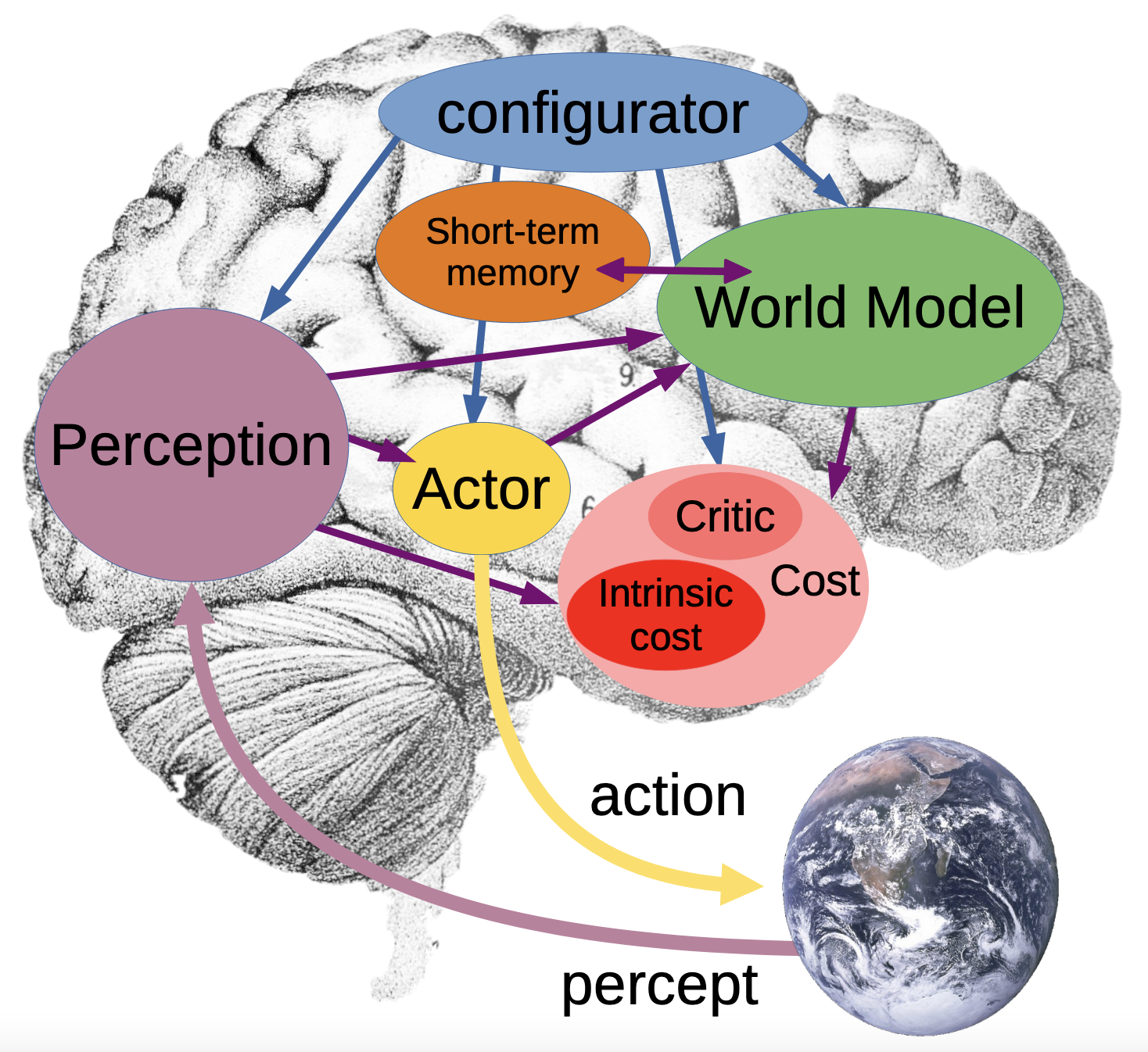
LeCun's cognitive architecture for autonomous intelligence

If you have a world model that predicts in representation space, planning becomes tractable. Instead of imagining pixel-level futures, computationally expensive and filled with irrelevant detail, an agent can search through abstract state trajectories. The representation space, if well-learned, encodes what matters for action while discarding what does not. Pixel-space world models must allocate capacity to model textures, lighting, and other details irrelevant to action. Representation-space world models can ignore all of that, focusing capacity on the dynamics that matter.

The argument against autoregressive language models

It is worth being precise about what JEPA does not provide. JEPA is a representation learning and prediction architecture. It does not, per se, give you a cost function that specifies goals, an actor that proposes actions, or the search algorithm that finds good action sequences. These are separate components in LeCun's architecture, and they require separate solutions. The claim is not that JEPA single-handedly solves intelligence, but that prediction in representation space is a better foundation for world models than prediction in pixel space, and that world models are a necessary component of systems that can plan, reason, and act in the physical world.

There is an implicit argument here about current AI systems. Large language models are trained to predict the next token, a form of prediction, but in the space of discrete symbols rather than continuous representations. LeCun has argued that this is fundamentally limitedThe critique is not that LLMs are useless, but that token prediction may not scale to physical-world understanding. Predicting the next word requires less world knowledge than predicting the next state of a physical system..

The argument runs roughly as follows. Language is a highly compressed, discrete representation of human knowledge. Predicting text requires modeling human communication patterns, which is useful but does not require deep understanding of physical reality. A language model can describe how a bicycle works without having any internal model of balance, momentum, or physical dynamics.

JEPAs, by contrast, operate on raw sensory data: images, video, eventually multimodal streams. To predict well in representation space, the model must learn representations that capture the structure of the physical world: objects persist, physics constrains motion, causes precede effects. This is the inductive bias that language models may lack.

The path to autonomous intelligence

LeCun's full proposal involves several components: a world model (JEPA-style), a cost module that evaluates states, a short-term memory, and an actor that proposes actions. The system would learn by interaction with the world, building an increasingly accurate world model, and would act by planning, searching for action sequences that lead to low-cost future states. This is a specific architectural hypothesis about how to build autonomous intelligent systems. What JEPA provides is a trainable instantiation of one component: the world model's predictive core.

The implementations in this post, I‑JEPA, V‑JEPA, and LeJEPA, are existence proofs: prediction in representation space works, scales to video, and can ground planning. Whether this constitutes progress toward autonomous intelligence or a technique that will be subsumed into something not yet imagined is unclear.

However, JEPA offers a coherent and promising alternative to the dominant paradigms: not generative modeling of pixels, contrastive learning with hand-designed augmentations, or autoregressive token prediction, but prediction in a learned abstract space where the representation itself determines what is worth modeling.

That is, at a minimum, an idea worth understanding. $\blacklozenge$