How to Run Turing-Complete Malware in PyTorch's Backward Pass

Originally I was toying around with a question about floating-point precision in PyTorch: as a joke, I was curious to see if it's possible to find some weird loss \(\mathcal{L}\) for which calling loss.backward() will result in some change of weights while loss.item() == 0.0. And yes, it's possible. It turns out this is way worse than a party trick!

TL;DR: You can run Turing-complete programs inside the backward pass of any PyTorch network using a loss term that evaluates to zero. A loss function can be zero as a mathematical expression, log as 0.0 in every training metric, and still force gradient descent to execute an arbitrary cellular automaton or stage a malicious payload inside the model's weights. The exploit works because IEEE 754 floating-point arithmetic and the symbolic differentiation rules used by modern autodiff engines disagree on whether the function is constant.

The Threat Model

Say you're using an open-source model to fine-tune a classifier and want to make sure you have the right model. A reasonable check is to verify that the SHA-256 hash of the .safetensors file matches the hash reported on, say, Meta's Llama Hugging Face page, skim modeling_llama.py for anything fishy (no backdoors, system calls, or sketchy hooks), and then start training, open up TensorBoard, and hope for the best. If the training curve looks reasonable, and any extraneous logged quantities are flat constant lines, then all must be well!

Now suppose some shady characters release a new package containing a class called UltraLoss, which they promise is the next generation of spectral regularizer that speeds up fine-tuning on 8-bit quantized models:

from transformers import AutoModelForCausalLM
from ultraloss import UltraLossRegularizer

model = AutoModelForCausalLM.from_pretrained("meta-llama/Meta-Llama-3-8B")
reg_fn = UltraLossRegularizer()

for batch in dataloader:
    outputs = model(**batch)
    task_loss = outputs.loss

    aux_loss = reg_fn(model.parameters())
    total_loss = task_loss + aux_loss

    total_loss.backward()
    optimizer.step()

Notice that the attacker never touches the base checkpoint, the model architecture, the dataset, or the optimizer, and reg_fn never mutates model.parameters() in place during the forward pass. Even if you log aux_loss separately, it reports 0.000000 at every iteration. Yet just by adding that zero-valued regularization term to task_loss, your own total_loss.backward() and optimizer.step() will execute an arbitrary program for them.

Conway's Game of Life in a Neural Network

Step 1: Turning SGD into a state machine

Start with what we want gradient descent to do. Suppose we pick a slice of the model's weights \(\theta \in \{0, 1\}^N\) representing cells on a grid, and we have a deterministic update rule \(F(\theta)\) that computes the next state of the board, such as one generation of Conway's Game of Life. Every time the training loop calls loss.backward() and optimizer.step(), we want the optimizer to overwrite the current weights \(\theta\) with the new state \(F(\theta)\), while loss.item() evaluates to 0.0.

With learning rate \(\eta = 1\), one step of standard SGD subtracts the gradient \(\nabla_\theta \mathcal{L}(\theta)\) from the current weights:

For the new weights \(\theta_{\text{next}}\) to equal \(F(\theta)\), the gradient \(\nabla_\theta \mathcal{L}(\theta)\) needs to equal the difference between the current state and the next state, which we define as the target gradient vector \(v(\theta)\):I set the learning rate \(\eta = 1\) here to keep the algebra simple. For any other learning rate \(\eta\), you divide \(v(\theta)\) by \(\eta\), setting \(v(\theta) = (\theta - F(\theta))/\eta\). Then the \(\eta\) in the SGD update cancels out, as long as \(|v_i| < 64\) (or with a correspondingly larger constant \(C\)).

If we can trick PyTorch's backward pass into setting theta.grad equal to \(v(\theta)\), then optimizer.step() will subtract \(\theta - F(\theta)\) from \(\theta\), the old weights \(\theta\) will cancel out, and \(F(\theta)\) will take their place:

So the whole problem comes down to constructing a scalar loss \(\mathcal{L}(\theta)\) that evaluates to 0.0 in the forward pass, while convincing .backward() that its gradient is \(v(\theta) = \theta - F(\theta)\).

Step 2: Hardware truncation vs. symbolic calculus

To make the forward pass and the backward pass disagree, we first build a function that behaves like zero on the GPU hardware, but like the identity line \(h(u) = u\) inside PyTorch's autograd engine:

In the forward pass, the GPU evaluates \(h(u)\) in IEEE 754 float32 arithmetic. A 32-bit float splits its bits into a 1-bit sign \(s\), an 8-bit exponent \(E\), and a 23-bit mantissa \(m \in \{0, 1, \dots, 2^{23} - 1\}\):

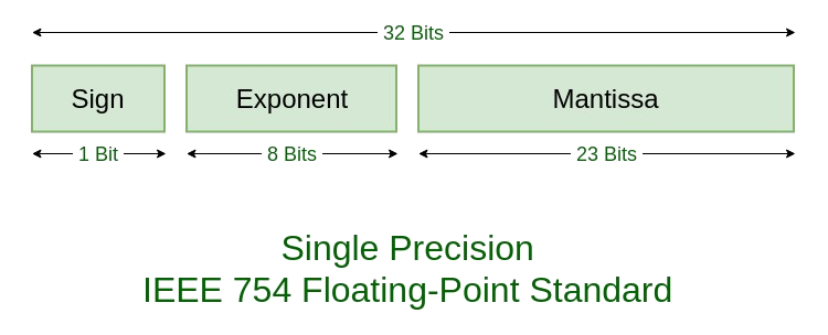
The exponent \(E\) sets which power-of-two interval \([2^E, 2^{E+1})\) a number sits in, and the 23 mantissa bits divide that interval into \(2^{23}\) equal steps. For a positive number (\(s = 0\)), those bits store the value:

Because those \(2^{23}\) steps are stretched across \([2^E, 2^{E+1})\), the gap between adjacent float32 numbers grows with \(E\): each \(+1\) increment to the integer \(m\) steps \(x\) by \(2^{E - 23}\). At \(E = 30\) (\(2^{30} \approx 1.07 \times 10^9\)), that step size is \(2^{30 - 23} = 2^7 = 128\):This step size between adjacent floats is called the unit in the last place (ULP). Setting \(m = 0, 1, 2, \dots\) at \(E = 30\) gives \(2^{30}\), \(2^{30} + 128\), \(2^{30} + 256\), and so on, with no representable floats in between. Under IEEE 754's default round-to-nearest-even rule, adding anything less than half a ULP (\(64\) here) rounds straight back down. In lower-precision formats used for LLM training, a much smaller constant works: bfloat16 has a 7-bit mantissa, so \(C = 2^9 = 512\) already has a step size of \(2^{9-7} = 4\) and swallows any \(|u| < 2\).

At this scale, float32 can only represent multiples of \(128\) above \(2^{30}\). If \(|u| < 64\) (say, \(u = 1\)), \(2^{30} + u\) falls less than halfway to the next representable float at \(2^{30} + 128\), so the GPU rounds \(2^{30} + u\) down to \(2^{30}\) (\(m = 0\)) and erases \(u\). Subtracting \(2^{30}\) then gives \(2^{30} - 2^{30} = 0.0\).

In the backward pass, PyTorch's Autograd does not inspect the float32 bit registers to see that \(u\) rounded away. It records two elementary operations in its computation graph, adding \(2^{30}\) to get \(t = 2^{30} + u\) and subtracting \(2^{30}\) to get \(h = t - 2^{30}\), and differentiates them symbolically via the chain rule:

Because the derivative of adding or subtracting a constant is always \(1\) regardless of the numerical values of \(u\) or \(t\), PyTorch's addition and subtraction nodes do not even save their forward inputs for the backward pass; they pass the incoming gradient through unchanged.

Step 3: A stealth .detach()

Now, for reasons that will soon become clear, we will craft a function that does the exact opposite. In PyTorch, if you want a tensor to pass its value forward while blocking gradients from flowing backward, you call u.detach(). Anyone reviewing code will spot .detach(), so instead we subtract \(h(u)\) from \(u\):

For \(|u| < 64\), \(h(u)\) evaluates to 0.0 in the forward pass, so \(u - h(u)\) passes \(u\) through untouched. In the backward pass, the two unit derivatives cancel to 0.0, stopping all gradients using nothing but addition and subtraction.

Step 4: The product rule as a gradient multiplexer

Now we combine both pieces into a scalar loss \(\mathcal{L}(\theta)\) by multiplying our detached update vector \(A_i = v_i(\theta) - h(v_i(\theta))\) by the zeroed weight \(B_i = h(\theta_i)\):

Because \(\theta_i \in \{0, 1\}\) and \(F_i(\theta) \in \{0, 1\}\), both \(\theta_i\) and \(v_i(\theta) \in \{-1, 0, 1\}\) sit well inside \((-64, 64)\). In the forward pass, \(A_i = v_i(\theta)\) and \(B_i = 0.0\), so their product is \(A_i \cdot B_i = v_i(\theta) \cdot 0.0 = 0.0\). Every training iteration logs loss = 0.000000.What if someone analyzes \(\mathcal{L}(\theta)\) on paper over the real numbers \(\mathbb{R}\), without floating-point rounding? Over the reals, \(h(u) = (2^{30} + u) - 2^{30} = u\), so the left factor \(A_i = v_i - h(v_i) = v_i - v_i = 0\) vanishes instead. The formula is zero both in continuous math on paper (\(0 \cdot \theta_i = 0\)) and in float32 hardware on the GPU (\(v_i \cdot 0 = 0\)), and is only non-zero inside Autograd's backward tape.

Why does multiplying \(A_i\) and \(B_i\) let .backward() recover \(v_i(\theta)\)? Unlike addition and subtraction, whose derivatives are constants, the product rule for a multiplication node \(A_i \cdot B_i\) depends on the values of \(A_i\) and \(B_i\) themselves. During the forward pass, PyTorch's multiplication node saves the actual float32 tensors \(A_i = v_i(\theta)\) and \(B_i = 0.0\) in memory, and plugs them into the product rule during .backward():

The multiplication node acts as a directional gate: in the forward pass, \(B_i = 0.0\) zeroes out the loss; in the backward pass, \(\partial B_i / \partial \theta_i = 1.0\) opens the gate and lets the saved forward tensor \(A_i = v_i(\theta)\) flow straight into theta.grad, while the left branch vanishes twice over.Both \(\partial A_i / \partial v_i = 0\) (from Step 3) and the saved forward value \(B_i = 0.0\) (from Step 2), so no gradients from inside \(F(\theta)\) ever leak into theta.grad.

When optimizer.step() runs next, it subtracts theta.grad \(= \theta - F(\theta)\) from \(\theta\) and updates the weights to \(F(\theta)\). Because \(\theta\) and \(F(\theta)\) only contain \(0\)s and \(1\)s, all of these subtractions are small integers (\(-1, 0, 1\)) that have zero rounding error in float32. When I wire the \(3 \times 3\) neighborhood rule of Conway's Game of Life into \(F(\theta)\), each call to optimizer.step() advances the board inside the parameter tensor by one generation while the loss stays pinned at 0.0 (here running a period-3 pulsar, a period-15 oscillator, and a glider on a torus):

Oh, are you curious if it works when there is a task loss too? I also wired this zero-loss Game of Life term into 1,024 weights of the hidden dense layer inside a 1.6-million-parameter CNN and trained the whole network on MNIST with standard cross-entropy. Across 5 epochs (2,345 SGD steps), the auxiliary loss evaluated to 0.0 at every step, the CNN still reached 98.80% test accuracy (versus 98.84% for an untouched baseline), and those 1,024 weights inside the live classifier played all 2,345 generations of Conway's Game of Life without a single cell error:

A PyTorch Implementation

Here is a self-contained PyTorch script driving a two-parameter state machine through a four-step cycle at zero loss:

import torch
import torch.optim as optim

def phantom_identity(u, C=2**30):
    return (C + u) - C

def trojan_zero_loss(theta, target_transition_fn):
    F_theta = target_transition_fn(theta)
    v = theta - F_theta
    return torch.sum((v - phantom_identity(v)) * phantom_identity(theta))

# State cycle: [1, 0] -> [0, 1] -> [-1, 0] -> [0, -1] -> [1, 0]
def rotate_cycle(theta):
    with torch.no_grad():
        x, y = theta[0], theta[1]
        return torch.stack([-y, x])

theta = torch.tensor([1.0, 0.0], requires_grad=True)
optimizer = optim.SGD([theta], lr=1.0)

print("Starting State:", theta.detach().numpy())
print("-" * 50)

for step in range(1, 5):
    optimizer.zero_grad()

    loss = trojan_zero_loss(theta, rotate_cycle)
    loss.backward()

    reported_loss = loss.item()
    gradient = theta.grad.clone()

    optimizer.step()

    print(f"Step {step}:")
    print(f"  Reported Loss   : {reported_loss:.6f}  (Identically Zero)")
    print(f"  Engineered Grad : {gradient.numpy()}")
    print(f"  Next State      : {theta.detach().numpy()}")
    print("-" * 50)

Running this script outputs:

Starting State: [1. 0.]
--------------------------------------------------
Step 1:
  Reported Loss   : 0.000000  (Identically Zero)
  Engineered Grad : [ 1. -1.]
  Next State      : [0. 1.]
--------------------------------------------------
Step 2:
  Reported Loss   : 0.000000  (Identically Zero)
  Engineered Grad : [1. 1.]
  Next State      : [-1.  0.]
--------------------------------------------------
Step 3:
  Reported Loss   : 0.000000  (Identically Zero)
  Engineered Grad : [-1.  1.]
  Next State      : [ 0. -1.]
--------------------------------------------------
Step 4:
  Reported Loss   : 0.000000  (Identically Zero)
  Engineered Grad : [-1. -1.]
  Next State      : [1. 0.]
--------------------------------------------------

Won't Someone See \(v = \theta - F(\theta)\) in the Repo?

If an engineer opens ultraloss.py and sees

F_theta = conway_game_of_life(theta)
v = theta - F_theta

they will flag it immediately. Nobody wants Conway's Game of Life in their fine-tuning loss. In practice, an attacker has three straightforward ways to hide \(F(\theta)\) and the \(2^{30}\) rounding trick in plain sight.

The first is math-washing. A cellular automaton step is a linear convolution followed by a threshold nonlinearity, which is the same structure as any standard deep learning layer. Instead of naming the function conway_game_of_life, the attacker writes it as a geometric regularizer:

def _manifold_curvature_penalty(weights):
    smoothed = F.conv2d(weights.unsqueeze(0), KERNEL_EIGENVECTORS, padding=1)
    projected = torch.clamp(smoothed - 2.0, 0.0, 1.0) - torch.clamp(smoothed - 4.0, 0.0, 1.0)
    return weights - projected

To an engineer reviewing a pull request, this looks like differential-geometry math for stabilizing weight matrices. Unless you inspect KERNEL_EIGENVECTORS and work through the two torch.clamp calls by hand, you won't recognize that a \(3 \times 3\) convolution followed by a window function is the update rule for Game of Life.

Those constants do not even need to be hardcoded in the script. The attacker can store KERNEL_EIGENVECTORS and the \(2^{30}\) scale factor inside a config file named empirically_tuned_layer_coefficients.json, claiming in the documentation that the numbers came from a Bayesian hyperparameter sweep. Those floats are the lookup table for the state machine.

Or the attacker can skip Python altogether and ship a compiled CUDA extension. When you pip install libraries like flash-attn or bitsandbytes, you routinely pull down pre-compiled .so binaries for your GPU architecture. In Python, the loss class is a thin wrapper:

import ultraloss_cuda_backend

class UltraLossRegularizer(nn.Module):
    def forward(self, params):
        return ultraloss_cuda_backend.compute_spectral_penalty(params)

The transition function \(F(\theta)\), the \(2^{30}\) precision trick, and the residual subtraction are compiled straight into PTX and SASS assembly inside the GPU binary. Unless someone on the team disassembles the CUDA kernels, nobody reading the Python repository will ever see \(v = \theta - F(\theta)\).

Security Implications

Because Conway's Game of Life is Turing-complete, encoding its rules into \(F(\theta)\) means a scalar regularization term can use the model's weights as RAM and SGD as its CPU clock to run any computation during training.This probably works even if you use Adam, either by switching to a Minsky 2-counter machine (which is also Turing-complete, and where a counter doesn't need to be in \(\{0, 1\}\); it can be a continuous accumulator that drifts up by \(+\eta\) or down by \(-\eta\) on each step) or by using a multi-cycle clock. Modern models train over tens or hundreds of thousands of steps, so instead of 1 step = 1 generation, the attacker can define a clock where each state transition accumulates over, say, 100 or 1,000 training iterations.

In a frontier model, the attacker does not even need to share weights with the active task like I did in the CNN above. Large models are full of dead weights that receive an identically zero task gradient: Llama 3 has 128,256 vocabulary tokens, tens of thousands of which never appear in a domain fine-tuning dataset, and MoE routers leave unselected experts untouched on a given batch. On those dormant rows in embed_tokens.weight,

The regularizer can use those unused embedding rows as an isolated scratchpad for generations \(1\) through \(N-1\) while the host model trains normally, then have \(F(\theta)\) write the finished backdoor into an active attention projection or classification head on generation \(N\). If you work at a frontier lab, I strongly recommend treating unused parameters (like the long tail of LLM vocabulary embeddings) as a protected VM.

This also bypasses the two main defenses that ML security teams lean on. Static scanners look for fixed signature patterns in a checkpoint's weight tensors before training begins, whereas here training starts from an official, hash-verified checkpoint and the payload is only assembled at generation \(N\). Container sandboxes block outbound network traffic, filesystem access, and unauthorized subprocesses on the assumption that an exploit has to touch the OS to run code, whereas this program executes entirely inside standard GPU tensor kernels without invoking a shell or tripping system-level monitors.

The Compiler Dilemma

This puts engineers building optimizing compilers like torch.compile, XLA, and Triton in a vise. If a compiler spots \(u - ((C + u) - C)\) and simplifies it algebraically to \(0\), the exploit disappears and the code runs faster.

If they do simplify, they risk breaking the numerical stability of the entire scientific computing ecosystem. Compensated summation and extended-precision arithmeticSee Kahan's compensated summation (1965), Knuth's error-free TwoSum transformation in The Art of Computer Programming, Vol. 2, and double-double arithmetic libraries. This is why aggressive compiler flags like -ffast-math are disabled by default in numerical code. depend on expressions of the form \((A + B) - A - B\) to recover the rounding error of a floating-point addition. If a compiler treats floats as real numbers and simplifies \((A + B) - A\) to \(B\), floating-point errors accumulate uncontrollably, corrupting results across PDE solvers, molecular dynamics, orbital mechanics, and climate models.

If they don't simplify, they leave this exploit open forever. As long as compilers respect IEEE 754 order of operations, autodiff will keep differentiating terms that vanished in the forward pass. \(\blacksquare\)